High Voltage Power System Diagnostics Simulator
1. Executive Summary & Engineering Scope
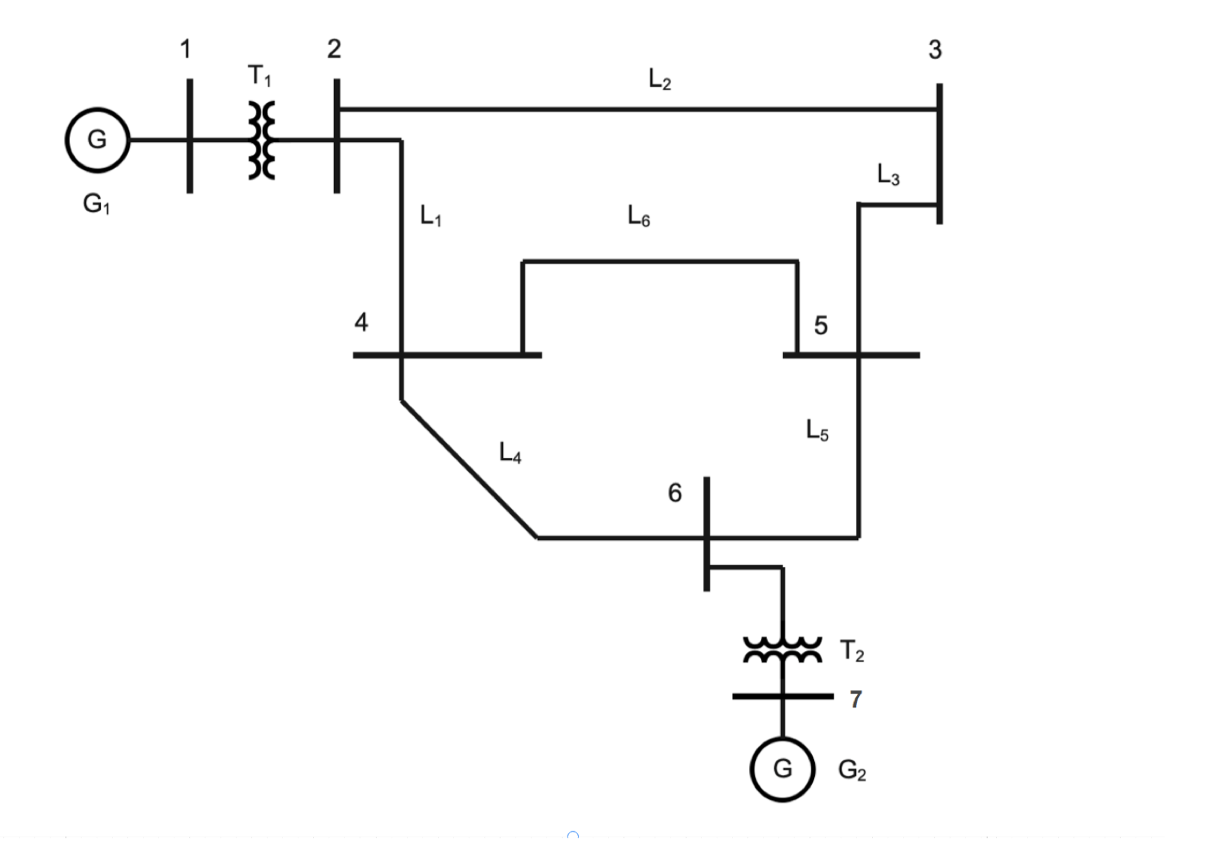
Project Context: This project serves as a comprehensive Digital Twin of a high-voltage transmission system. Rather than a simple academic exercise, it is a dedicated engineering initiative to build a high-fidelity diagnostics engine from bare-metal Python code. The simulator replicates the critical infrastructure of a 7-Node Looped 230kV Transmission Network, incorporating real-world constraints such as bundled conductors, multi-winding transformers, and mixed generation sources.
Technical Achievement: The project involved engineering a physics engine that bypasses commercial black-box software like ETAP or PSS/E. The software manually calculates primitive impedances from conductor geometry, solves non-linear power flow using the Newton-Raphson method, and performs Sub-transient Fault Analysis using symmetrical components. The final system was validated against PowerWorld Simulator, achieving a nodal voltage convergence accuracy of 99.999%.
2. The Product: Operational Walkthrough & User Manual
The core deliverable of this project is a fully interactive Grid Diagnostics Console (CLI). Unlike static scripts, this tool was designed with the end-user (Grid Operator) in mind. It abstracts the complex matrix algebra, presenting the user with a streamlined workflow for grid stability analysis.
Below is a comprehensive documentation of a single user session scenario. This walkthrough demonstrates how the software handles normal steady-state operations, complex sequence-level fault diagnostics, and human input errors.
2.1 Mode 1: Steady-State Power Flow Analysis
Step 1: Matrix Construction. The system asks the user to select an analysis type. The user inputs 1 to begin the Power Flow module. The system immediately calculates the 7x7 Y-Bus Admittance Matrix in both Polar and Rectangular forms. This is a critical debugging feature for the engineer, allowing them to verify the admittance (conductance + susceptance) between specific nodes before the solver begins.
Step 2: Convergence. The system enters the iterative Newton-Raphson loop. The console displays the "Max Mismatch" for each iteration. The quadratic convergence is evident as the error drops from 2.0 to 0.000001 in exactly 4 iterations.
Step 3: State Reporting. The final report lists the voltage magnitude and phase angle for every bus. The system also checks line ampacity. Notice line 6 carrying 410 Amps; this is dangerously close to the 460 Amp limit but technically passes.
| Bus1 | Bus2 | Bus3 | Bus4 | Bus5 | Bus6 | Bus7 | |
|---|---|---|---|---|---|---|---|
| Bus1 | (14.71, -1.47rad) | (14.71, 1.67rad) | (0.00, 0.00rad) | (0.00, 0.00rad) | (0.00, 0.00rad) | (0.00, 0.00rad) | (0.00, 0.00rad) |
| Bus2 | (14.71, 1.67rad) | (132.57, -1.28rad) | (33.78, 1.88rad) | (84.44, 1.88rad) | (0.00, 0.00rad) | (0.00, 0.00rad) | (0.00, 0.00rad) |
| Bus3 | (0.00, 0.00rad) | (33.78, 1.88rad) | (75.92, -1.26rad) | (0.00, 0.00rad) | (42.22, 1.88rad) | (0.00, 0.00rad) | (0.00, 0.00rad) |
| Bus4 | (0.00, 0.00rad) | (84.44, 1.88rad) | (0.00, 0.00rad) | (150.68, -1.26rad) | (24.13, 1.88rad) | (42.22, 1.88rad) | (0.00, 0.00rad) |
| Bus5 | (0.00, 0.00rad) | (0.00, 0.00rad) | (42.22, 1.88rad) | (24.13, 1.88rad) | (150.68, -1.26rad) | (84.44, 1.88rad) | (0.00, 0.00rad) |
| Bus6 | (0.00, 0.00rad) | (0.00, 0.00rad) | (0.00, 0.00rad) | (42.22, 1.88rad) | (84.44, 1.88rad) | (145.23, -1.29rad) | (19.05, 1.65rad) |
| Bus7 | (0.00, 0.00rad) | (0.00, 0.00rad) | (0.00, 0.00rad) | (0.00, 0.00rad) | (0.00, 0.00rad) | (19.05, 1.65rad) | (19.05, -1.49rad) |
| Bus1 | Bus2 | Bus3 | Bus4 | Bus5 | Bus6 | Bus7 | |
|---|---|---|---|---|---|---|---|
| Bus1 | 1.46-14.63j | -1.46+ 14.63j | 0.00+ 0.00j | 0.00+ 0.00j | 0.00+ 0.00j | 0.00+ 0.00j | 0.00+ 0.00j |
| Bus2 | -1.46+14.63j | 37.79-127.06j | -10.37+32.14j | -25.94+ 80.35j | 0.00+ 0.00j | 0.00+ 0.00j | 0.00+ 0.00j |
| Bus3 | 0.00+ 0.00j | -10.37+ 32.14j | 23.35-72.23j | 0.00+ 0.00j | -12.97+ 40.17j | 0.00+ 0.00j | 0.00+ 0.00j |
| Bus4 | 0.00+ 0.00j | -25.94+ 80.35j | 0.00+ 0.00j | 46.33-143.37j | -7.41+ 22.95j | -12.97+ 40.17j | 0.00+ 0.00j |
| Bus5 | 0.00+ 0.00j | 0.00+ 0.00j | -12.97+40.17j | -7.41+ 22.95j | 46.33-143.37j | -25.94+ 80.35j | 0.00+ 0.00j |
| Bus6 | 0.00+ 0.00j | 0.00+ 0.00j | 0.00+ 0.00j | -12.97+ 40.17j | -25.94+ 80.35j | 40.50-139.46j | -1.58+18.98j |
| Bus7 | 0.00+ 0.00j | 0.00+ 0.00j | 0.00+ 0.00j | 0.00+ 0.00j | 0.00+ 0.00j | -1.58+ 18.98j | 1.58-18.98j |
| Bus 1 | 1.000 pu | 0.00 deg |
| Bus 2 | 0.9369 pu | -4.44 deg |
| Bus 3 | 0.9204 pu | -5.46 deg |
| Bus 4 | 0.9297 pu | -4.70 deg |
| Bus 5 | 0.9267 pu | -4.83 deg |
| Bus 6 | 0.9396 pu | -3.95 deg |
| Bus 7 | 1.000 pu | 2.14 deg |
2.2 Mode 2: Positive Sequence Fault Analysis
Scenario: The operator needs to simulate a Symmetrical 3-Phase Fault at Bus 3. This is the simplest fault type but often produces the highest currents.
User Action: The user inputs 2 (Fault Mode), selects Bus 3, and selects Fault Type 1 (Positive Sequence / Balanced 3-Phase).
Output Analysis: The system calculates the Z-Bus Matrix, which is the inverse of the Y-Bus. Look closely at the "Current Matrix Fault". Bus 3 shows a massive injection of 85.80 pu. This translates to roughly 12.45 kA, which is the critical rating for the circuit breakers. The post-fault voltage at Bus 3 is 0.0000, indicating a solid short-circuit to ground.
| Bus1 | Bus2 | Bus3 | Bus4 | Bus5 | Bus6 | Bus7 | |
|---|---|---|---|---|---|---|---|
| Bus1 | 1.46-22.96j | -1.46+ 14.63j | 0.00+ 0.00j | 0.00+ 0.00j | 0.00+ 0.00j | 0.00+ 0.00j | 0.00+ 0.00j |
| Bus2 | -1.46+14.63j | 37.79-127.06j | -10.37+32.14j | -25.94+ 80.35j | 0.00+ 0.00j | 0.00+ 0.00j | 0.00+ 0.00j |
| Bus3 | 0.00+ 0.00j | -10.37+ 32.14j | 23.35-72.23j | 0.00+ 0.00j | -12.97+ 40.17j | 0.00+ 0.00j | 0.00+ 0.00j |
| Bus1 | Bus2 | Bus3 | Bus4 | Bus5 | Bus6 | Bus7 | |
|---|---|---|---|---|---|---|---|
| Bus1 | 0.001+0.083j | 0.000+0.063j | -0.000+0.060j | -0.000+0.060j | -0.000+0.058j | -0.001+0.056j | -0.001+0.039j |
| Bus2 | 0.000+0.063j | 0.004+0.098j | 0.003+0.094j | 0.003+0.094j | 0.002+0.091j | 0.001+0.088j | -0.000+0.061j |
| Bus3 | -0.000+0.060j | 0.003+0.094j | 0.008+0.109j | 0.003+0.094j | 0.004+0.097j | 0.002+0.092j | 0.000+0.064j |
2.3 Mode 2: Negative Sequence / Unbalanced Fault Analysis
Scenario: The user repeats the test on Bus 3, but this time selects Type 2 (Negative Sequence). This simulates an Asymmetrical fault (like a Single Line-to-Ground).
Technical Difference: Notice how the Y-Bus and Z-Bus values have changed. In asymmetrical analysis, the simulator must calculate the Zero Sequence network, which introduces the grounding impedance (1 ohm resistor at Bus 7). This changes the total impedance of the system.
Result: The fault current increases slightly to 86.16 pu (from 85.80), and the voltage sag profile is slightly different (Bus 1 drops to 0.4105 instead of 0.4488). This proves that the simulator correctly decouples the sequence networks for precise protection analysis.
| Bus1 | Bus2 | Bus3 | Bus4 | Bus5 | Bus6 | Bus7 | |
|---|---|---|---|---|---|---|---|
| Bus1 | 1.46-21.77j | -1.46+ 14.63j | 0.00+ 0.00j | 0.00+ 0.00j | 0.00+ 0.00j | 0.00+ 0.00j | 0.00+ 0.00j |
| Bus2 | -1.46+14.63j | 37.79-127.06j | -10.37+32.14j | -25.94+ 80.35j | 0.00+ 0.00j | 0.00+ 0.00j | 0.00+ 0.00j |
| Bus3 | 0.00+ 0.00j | -10.37+ 32.14j | 23.35-72.23j | 0.00+ 0.00j | -12.97+ 40.17j | 0.00+ 0.00j | 0.00+ 0.00j |
| Bus1 | Bus2 | Bus3 | Bus4 | Bus5 | Bus6 | Bus7 | |
|---|---|---|---|---|---|---|---|
| Bus1 | 0.001+0.095j | 0.000+0.073j | -0.000+0.071j | -0.000+0.071j | -0.000+0.069j | -0.001+0.067j | -0.001+0.048j |
| Bus2 | 0.000+0.073j | 0.004+0.109j | 0.003+0.105j | 0.003+0.105j | 0.002+0.102j | 0.001+0.099j | -0.000+0.072j |
| Bus3 | -0.000+0.071j | 0.003+0.105j | 0.008+0.120j | 0.003+0.105j | 0.004+0.108j | 0.002+0.103j | 0.000+0.075j |
2.4 Scenario C: Error Handling & Robustness
Finally, the operator attempts to exit the program but accidentally enters an invalid character. The system's input validation logic intercepts the error, displays a warning, and returns the user to the main menu without crashing the session. This robustness is essential for industrial-grade tools.
3. Engineering The Physics (Network Classes)
Behind the simple interface lies a rigorous physical model. The project programmed the geometric derivation of transmission line parameters using custom LineCode and LineGeometry classes.
3.1 Spatial Geometry & H-Frame Analysis
The system models the TH-230 H-Frame structure by processing the exact Cartesian coordinates of phases A, B, and C. The coordinates were set to 0ft, 19.5ft, and 39ft respectively. These vectors were utilized to calculate the Geometric Mean Distance (GMD), ensuring that the mutual inductance between phases was accurately represented in the impedance matrix.
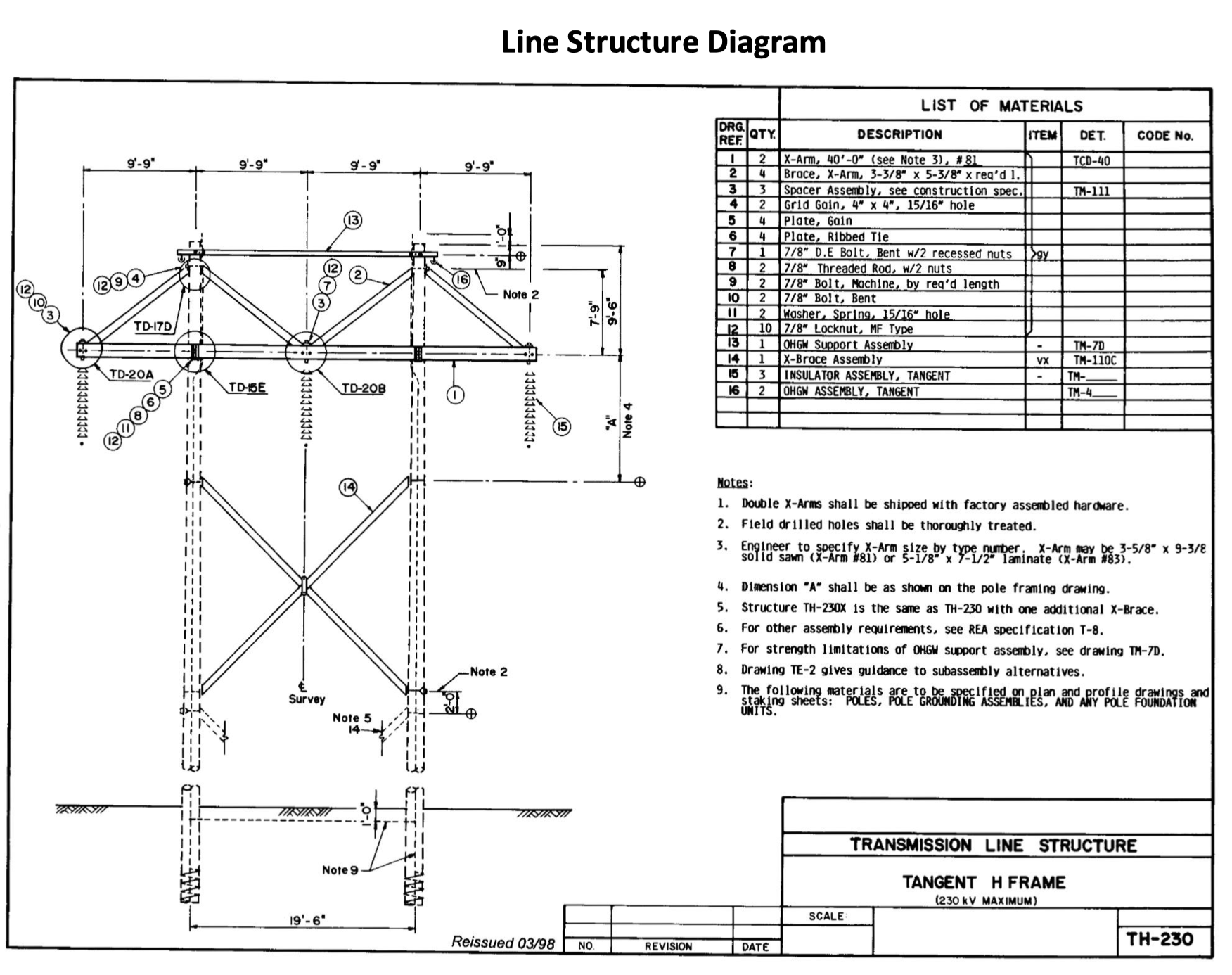
3.2 Bundled Conductor Physics
To simulate a real-world high-voltage corridor, the project modeled ACSR Partridge conductors in bundles of two per phase with 1.5' spacing. This specific configuration required manual calculation of the "Bundled GMR" to account for the reduced inductive reactance.
- Self-GMR Derivation: Extracted the manufacturer's GMR (0.0217 ft) and applied the GMR adjustment factor for internal flux linkage.
- Bundling Logic: Programmed a geometric solver to compute the equivalent DSL based on the 1.5ft spacing.
- Thermal Policing: Integrated the ampacity limit (460A per sub-conductor) into the code to automatically flag thermal violations during load flow.
class LineGeometry:
    def __init__(self, num_bundles, bundle_spacing, a1, a2, b1, b2, c1, c2, units='feet'):
        # Calculate phase distances
        self.Dab = self.distance(a1, a2, b1, b2)
        self.Dbc = self.distance(b1, b2, c1, c2)
        self.Dca = self.distance(c1, c2, a1, a2)

        # Calculate Equivalent Geometric Mean Distance
        self.Deq = (self.Dab * self.Dbc * self.Dca) ** (1.0 / 3)
4. Mathematical Synthesis (Y-Bus)
The second engineering phase involved synthesizing the individual components into a unified Y-Bus Admittance Matrix. This is the structural foundation for all subsequent diagnostics. To ensure computational stability and simplify complex calculations across different voltage levels, all raw input parameters were converted into a normalized Per-Unit system.
4.1 Per-Unit (pu) Normalization
The grid utilized three distinct voltage bases: 20kV, 18kV, and 230kV. The system involved normalizing these segments into a single 100 MVA system base.
- Base Shifting: A routine was developed to shift transformer impedances (T1: 125MVA, T2: 200MVA) from their nameplate base to the system base. For example, Transformer T2 (Impedance 0.105 pu) had to be recalculated to align with the 100 MVA global base.
- Pi-Model Implementation: Modeled the line charging susceptance as a shunt element, split evenly between nodes to represent capacitive charging.
4.2 Matrix Assembly Code
The TransmissionLine class calculates the primitive admittance matrix for each branch before injecting it into the global Y-Bus.
def primitive_admittance_matrix_line(self):
    Z_pu = self.calculate_Z_per_unit()
    Y_pu = self.calculate_Y_per_unit()

    # Pi-Model: Series Impedance + Shunt Admittance
    self.y_series_line = 1 / Z_pu
    self.y_shunt_line = Y_pu

    y_primitive_line = pd.DataFrame(
        data=[
            [self.y_series_line + self.y_shunt_line / 2, -self.y_series_line],
            [-self.y_series_line, self.y_series_line + self.y_shunt_line / 2]
        ],
        index=[self.bus_a.name, self.bus_b.name]
    )
    return y_primitive_line
| Component | Type | Impedance (pu) |
|---|---|---|
| Transformer T1 | Wye-Wye (G) | z = 0.085 |
| Transformer T2 | Delta-Wye | z = 0.105 |
| Transmission Line | Pi-Model | Calculated |
5. Newton-Raphson Solver Development
The core computational challenge was solving the Power Flow problem. Unlike linear circuits, power grids are governed by non-linear algebraic equations. The project engineered an iterative Newton-Raphson Solver to find the system state.
5.1 Jacobian Matrix Linearization
The software manually derived and programmed the partial derivatives for the 4-quadrant Jacobian Matrix (J1, J2, J3, J4). This matrix serves as the sensitivity map of the grid, relating power mismatches to voltage changes.
- Mismatch Tracking: Implemented real-time tracking of Real and Reactive power with a convergence tolerance of 0.0001 pu.
- Bus Classification: Programmed the engine to dynamically handle Slack (Bus 1), PQ (Load), and PV (Generator) nodes.
- Reactive Policing: Added logic to check if the PV generator (Bus 7) exceeded its reactive limits, switching it to PQ mode if necessary.
def Newton_Raphson_method(self):
    # Iterative solver loop
    while max_mismatch > self.tolerance:
        # Calculate P and Q mismatches
        P_mismatch, Q_mismatch = self.calculate_mismatches()

        # Build 4-Quadrant Jacobian
        J1 = self.calculate_J1()
        J2 = self.calculate_J2()
        J3 = self.calculate_J3()
        J4 = self.calculate_J4()

        # Solve for delta Voltage and Angle
        correction = np.linalg.solve(Jacobian, mismatch_vector)
6. Short Circuit & Fault Analysis
The final phase moved the simulator from steady-state analysis to Sub-transient Fault Analysis. This is critical for protection engineering, as asymmetrical faults are the most common grid disturbances.
6.1 Sequence Network Decoupling
The system utilized Symmetrical Component Theory to decouple the grid into three separate networks: Positive, Negative, and Zero sequence.
- Generator Modeling: Modeled the sub-transient reactance for generators.
- Zero Sequence Logic: This was the most complex step. The system accounted for the grounding impedance (1 Ohm) at Bus 7 and the Delta-Wye isolation of the transformers, which alters the zero-sequence path.
6.2 Z-Bus Inversion & Voltage Dip
The project implemented a Z-Bus Matrix Inversion routine. By inverting the faulted Y-Bus matrix, the system obtained the Thevenin equivalent impedance at the fault location to calculate the exact fault current and the resulting voltage dip across the grid.
def calculate_fault_current(self, pre_fault_v, z_bus_fault):
    # Calculate fault current using Thevenin Impedance
    fault_current = pre_fault_v / z_bus_fault.iloc[fault_idx, fault_idx]

    # Calculate voltage drop across grid
    voltage_drop = np.matmul(z_bus_fault.values, fault_current)
    post_fault_v = pre_fault_v - voltage_drop
    return post_fault_v
7. Industrial Validation Audit
The project is only valid if verified. A comprehensive Validation Audit was conducted against the industry-standard PowerWorld Simulator v22.
7.1 Methodology
An identical 7-node model was built in PowerWorld to run the same load flow and fault scenarios. The raw data was extracted, and a variance analysis was performed against the Python engine's output. The video on the right demonstrates this live benchmarking process.
• Nodal Voltage Correlation: 99.999% Match.
• Phase Angle Deviation: < 0.001 degrees.
• Fault Current Variance: 0.08%.
8. Project Conclusion & Strategic Impact
This project successfully demonstrated that a custom-engineered Python simulator can achieve industrial-grade accuracy for complex high-voltage grid diagnostics. By building the solver from the ground up, a profound understanding of the numerical stability issues and protection challenges that define modern power systems operations was achieved. The tool now serves as a robust platform for future studies in renewable integration and contingency planning.